Clustering vs. Mean-Variance Optimization: An Empirical Study of Diversification Performance and Risk

Introduction

Diversification is a fundamental concept in the world of investing. As the old adage goes, “Don’t put all your eggs in one basket.” Portfolio diversification involves spreading investments across different assets to reduce risk and improve returns. It’s crucial for investors to avoid overexposure to any single asset and mitigate potential losses.

**Clustering **and mean-variance optimization (MVO) are two popular approaches for diversification — clustering groups similar-performing assets, while MVO optimizes portfolio weights for risk-return trade-offs.

In this article, we will assess the effectiveness of clustering and mean-variance optimization (MVO) in enhancing risk-adjusted returns. Through empirical analysis, we will evaluate each strategy’s performance metrics, including Sharpe ratio, annualized volatility and cumulative returns. This will help us to understand the underlying tradeoffs between these strategies.

Methodology

For our empirical analysis of diversification performance and risk of the two methods, we will follow the following methodology:

1. Data Collection: We will collect returns data for a sample selection of 50 tickers from the S&P 500. The stocks have been selected across a variety of sectors. The data will be from 2010–01–01 to 2023–01–01.

2. Portfolio Construction: The next step is to construct portfolios for our stocks using our diversification strategies. This involves calculating weights by implementing the strategy.

3. Performance Metrics: We will use a pre-defined set of performance metrics to evaluate risk and return characteristics of each portfolio. We will use the following metrics: Sharpe ratio, annualized volatility and cumulative returns.

Mean-Variance Optimization

Modern Portfolio Theory is a mathematical framework introduced by Harry Markowitz that focuses on diversification and risk-return trade-offs. It involves constructing a portfolio based on the expected returns, variances, and covariances of the assets.

Mean-Variance Optimization (MVO) is a key technique in Modern Portfolio Theory — used to construct an efficient frontier, which represents optimal portfolios that offer the highest expected return for a given level of risk.

An example of an Efficient Frontier graph [Image source: QuantPy]

Methodology

Step 1: Creating the covariance matrix

By observing how different assets have performed in the past, we can calculate their mean (average) returns and assess how they fluctuate relative to one another. The latter is achieved through the covariance matrix — a mathematical tool that quantifies how assets move together.

Calculate mean returns and covariance matrix

mean_returns = df_stock_returns.mean() cov_matrix = df_stock_returns.cov() cov_matrix

Plot the covariance matrix using a heatmap

plt.figure(figsize=(8, 6)) sns.heatmap(cov_matrix, annot=False, cmap='coolwarm', fmt='.6f', cbar=False) plt.title('Covariance Matrix') plt.show()

To better understand how assets interact, we can create a heatmap of the covariance matrix. In this visual representation, each cell represents the covariance between a pair of assets. A heatmap allows us to quickly identify which assets tend to move together and which move in opposite directions.

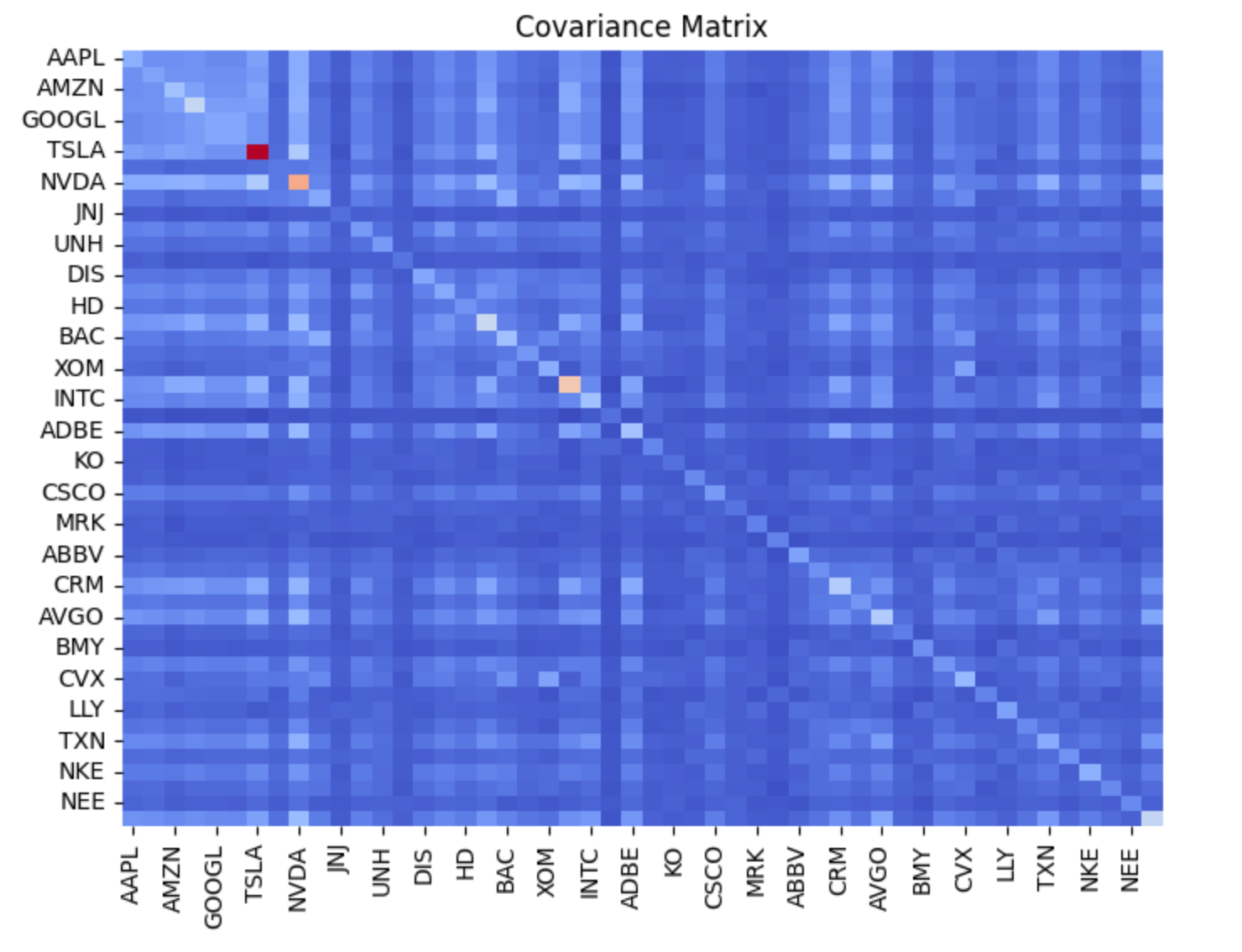Generated covariance matrix

Step 2: Defining optimization objective

The crux of MVO is defining an objective to be optimized. The objective function measures the portfolio’s risk, often expressed as volatility (a measure of how returns fluctuate over time). Our goal is to find the asset allocation that minimizes this risk while meeting certain constraints.

def calculate_portfolio_volatility(weights, cov_matrix): """ Calculate the volatility of a portfolio given the asset weights and covariance matrix. """ return np.sqrt(weights.T @ cov_matrix @ weights)

Number of assets in the portfolio

num_assets = len(mean_returns)

Define the objective function (minimize portfolio volatility)

objective_function = lambda weights: calculate_portfolio_volatility(weights, cov_matrix)

Step 3: Setting Constraints

Investment portfolios are subject to various constraints. For example, the sum of all asset weights should equal 100% (fully invested). Additionally, we may restrict short-selling by ensuring that all asset weights are non-negative.

Define the constraints

Constraint 1: The sum of the weights must be equal to 1 (fully invested)

Constraint 2: The weights must be between 0 and 1 (no short-selling)

constraints = ({'type': 'eq', 'fun': lambda weights: np.sum(weights) - 1})
bounds = [(0, 1) for i in range(num_assets)]

Step 4: Running the optimization and computing the weights

With the objective function and constraints defined, we can use an optimization algorithm to find the asset allocation that best meets our criteria. The result is a set of optimal portfolio weights.

from scipy.optimize import minimize

Initialize equal weights for the optimization starting point

initial_weights = np.repeat(1/num_assets, num_assets)

Perform the optimization

result = minimize( objective_function, initial_weights, bounds=bounds, constraints=constraints, method='SLSQP' )

Extract the optimal weights from the optimization result

optimal_weights = result.x df_weights = pd.Series(optimal_weights, index=df_stock_returns.columns, name='Optimal Weights') print(df_weights)

Great! Now we have the weights for Mean-Variance optimization. Let’s proceed with the hierarchical clustering method and compute its weights before we compare their performance.

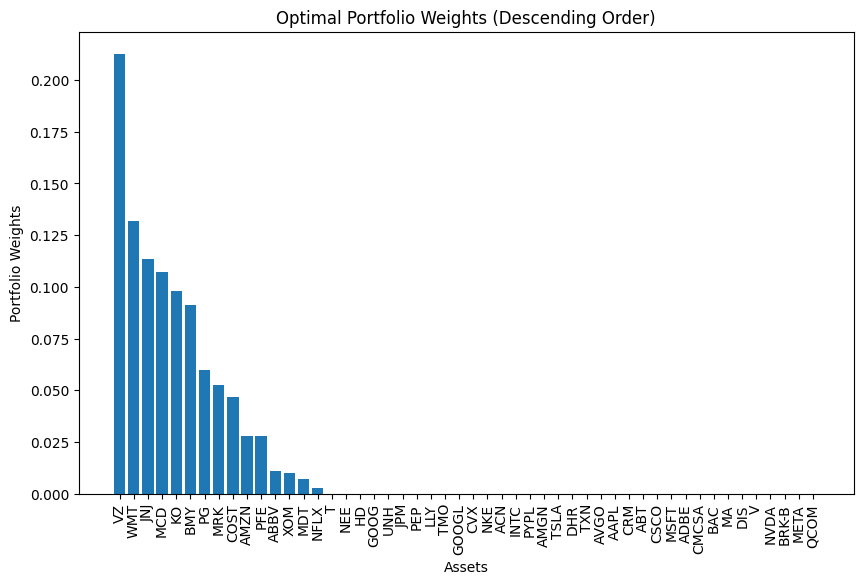Optimal Portfolio Weights (Mean Variance Optimization)

Clustering

Clustering is a machine learning technique used to group similar objects or data points based on their characteristics or features. Three commonly used clustering algorithms are K-means clustering, hierarchical clustering, and DBSCAN.

K-Means Clustering

K-means aims to minimize the within-cluster variance:

where

• J(μ) is the objective function to be minimized.

• *K *is the number of clusters.

• C_k ​is the set of data points belonging to cluster.

• x_i ​is a data point.

• μ_k ​is the centroid of cluster k

It requires pre-specification of K and assumes spherical and equally-sized clusters.

Hierarchical Clustering

Hierarchical clustering builds a tree-like structure (dendrogram) by recursively merging (agglomerative) or splitting (divisive) clusters based on a distance or similarity measure (e.g., Euclidean distance).

The distance between clusters can be calculated using linkage methods such as single-linkage, complete-linkage, or average-linkage.

There is no need to pre-specify the number of clusters; the dendrogram allows selecting the desired level of granularity.

DBSCAN (Density-Based Spatial Clustering of Applications with Noise)

DBSCAN groups points based on density by defining a neighborhood radius (ε) and a minimum number of points to form a dense region.

A cluster is formed by connecting points within the ε-neighborhood, and noise points are identified as those not belonging to any cluster.

It is capable of handling clusters of arbitrary shapes and sizes, and robust to outliers.

Selection of a Clustering Algorithm

Hierarchical clustering is the preferred clustering algorithm for portfolio diversification because of its ability to capture complex relationships between assets and its flexibility in determining the number of clusters.

• The dendrogram provides insights into asset correlations and allows for selecting representative assets from distinct clusters to achieve effective diversification.

• Additionally, hierarchical clustering can handle non-spherical clusters and varying densities, which are advantageous when dealing with stock return data that exhibit diverse patterns.

Hierarchical Clustering Methodology

Hierarchical Risk Parity is a portfolio construction approach introduced by Marcos López de Prado. HRP offers a robust and intuitive way to allocate assets based on their hierarchical relationships. Unlike traditional risk parity, HRP accounts for the hierarchical structure of asset correlations, creating more diversified and risk-balanced portfolios.

Step 1: Computing the Linkage Matrix

The foundation of HRP is hierarchical clustering — a method that groups assets based on their similarities. We start by computing a linkage matrix, which describes the hierarchical relationships among assets. Assets that exhibit similar return patterns are clustered together, forming a tree-like structure called a dendrogram.

from scipy.cluster.hierarchy import dendrogram, linkage from sklearn.preprocessing import StandardScaler import matplotlib.pyplot as plt

Standardize the returns data

scaler = StandardScaler() standardized_returns = scaler.fit_transform(df_stock_returns)

Perform hierarchical clustering using the Ward's linkage method

linkage_matrix = linkage(standardized_returns.T, method='ward')

Plot the dendrogram

plt.figure(figsize=(12, 6)) dendrogram(linkage_matrix, labels=df_stock_returns.columns, leaf_rotation=90) plt.title('Dendrogram of Hierarchical Clustering for Stock Returns') plt.xlabel('Stocks') plt.ylabel('Euclidean Distance') plt.show()

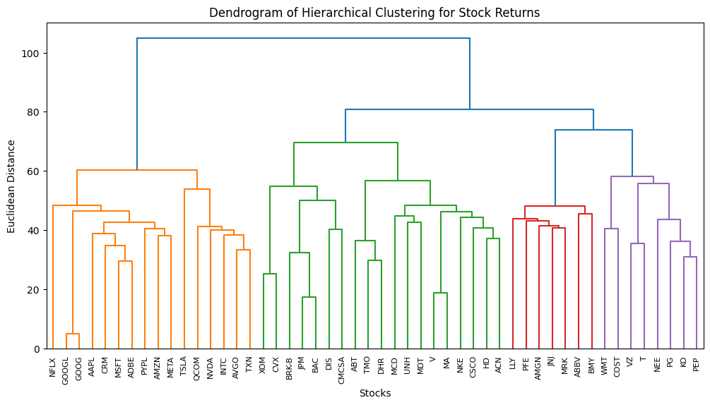Dendrogram of Hierarchical Clustering for Stock Returns

Step 2: Quasi-Diagonalization

Next, we reorder the covariance matrix of asset returns to reflect the hierarchical structure from the linkage matrix. This process is called quasi-diagonalization. By rearranging the matrix, assets that are closely related in the hierarchical clustering are placed close together. This step is crucial for achieving effective risk diversification.

def get_quasi_diagonalized_order(linkage_matrix): """ Returns the order of columns to quasi-diagonalize the covariance matrix. """

Get the linkage matrix as a list of pairs of clusters that were merged

cluster_pairs = linkage_matrix[:, :2].astype(int)

Define a function to recursively extract the original indices

def extract_original_indices(pair): left, right = pair if left < n_assets: yield int(left) else: yield from extract_original_indices(cluster_pairs[left - n_assets]) if right < n_assets: yield int(right) else: yield from extract_original_indices(cluster_pairs[right - n_assets])

n_assets = len(linkage_matrix) + 1 ordered_indices = list(extract_original_indices(cluster_pairs[-1])) return ordered_indices

Get the ordered indices for quasi-diagonalization from the linkage matrix

ordered_indices = get_quasi_diagonalized_order(linkage_matrix)

Reorder the covariance matrix based on the hierarchical clustering structure

cov_matrix = df_stock_returns.cov() # Calculate the covariance matrix of asset returns cov_matrix_quasi_diag = cov_matrix.iloc[ordered_indices, ordered_indices]

Display the quasi-diagonalized covariance matrix

cov_matrix_quasi_diag.head()

Step 3: Recursive Bisection

With the reordered covariance matrix, we proceed to allocate capital to assets using recursive bisection. Starting from the top of the hierarchy, we recursively apply risk parity allocation to each cluster, working our way down to individual assets. The goal is to equalize the risk contributions from each asset or cluster to the overall portfolio risk. At the end, we get the portfolio weights

import numpy as np

def get_inverse_variance_weights(cov_matrix): """ Compute inverse-variance portfolio weights based on the covariance matrix. """ inverse_variance = 1 / np.diag(cov_matrix) return inverse_variance / inverse_variance.sum()

def get_recursive_bisection_weights(linkage_matrix, cov_matrix, n_assets): """ Compute portfolio weights using recursive bisection based on the hierarchical structure. """

Initialize weights for all assets

weights = np.ones(n_assets)

Define a function to recursively apply risk parity allocation

def allocate(cluster_indices): if len(cluster_indices) > 1:

Extract the covariance matrix for the current cluster

cluster_cov = cov_matrix.iloc[cluster_indices, cluster_indices]

Calculate inverse-variance weights for the current cluster

cluster_weights = get_inverse_variance_weights(cluster_cov)

Update the weights based on risk contribution from each asset in the current cluster

weights[cluster_indices] *= cluster_weights

Recursively allocate weights to sub-clusters

left_indices = linkage_matrix[:, 2] == len(cluster_indices) left_cluster = linkage_matrix[left_indices, 0].astype(int) allocate(left_cluster)

right_indices = linkage_matrix[:, 2] == len(cluster_indices) right_cluster = linkage_matrix[right_indices, 1].astype(int) allocate(right_cluster)

Start the recursive bisection process from the top level of the hierarchy

top_level_indices = range(n_assets) allocate(top_level_indices)

Normalize the final weights so that they sum to one

return weights / weights.sum()

Compute portfolio weights using recursive bisection based on hierarchical clustering and covariance matrix

portfolio_weights = get_recursive_bisection_weights(linkage_matrix, cov_matrix_quasi_diag, len(df_stock_returns.columns))

Display the final portfolio weights for each asset

portfolio_weights_df = pd.Series(portfolio_weights, index=df_stock_returns.columns, name='Portfolio Weights') print(portfolio_weights_df.sum()) portfolio_weights_df.head()

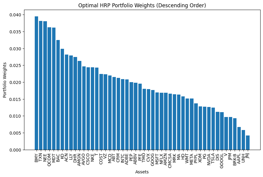Optimal HRP Portfolio Weights

Performance Metrics

After constructing the portfolios, we need to evaluate performance metrics. These performance metrics provide valuable insights into the portfolio’s behavior under various market conditions and allow investors to assess the effectiveness of their investment strategy.

Sharpe Ratio

The Sharpe Ratio is calculated as the excess return of the portfolio (above the risk-free rate) divided by its volatility. A higher Sharpe Ratio indicates better risk-adjusted performance.

Annualized Volatility

Another important metric is annualized volatility, which quantifies the degree of fluctuation in the portfolio’s returns over time. Lower annualized volatility suggests a more stable return profile, which is desirable for risk-averse investors.

Cumulative Return

Cumulative return reflects the overall growth of the portfolio over time. By plotting the portfolio’s cumulative returns, investors can visually assess how the investment would have performed historically.

We can calculate the performance metrics as follows:

Mean-Variance Optimization

Calculate the daily returns of the portfolio

portfolio_returns = df_stock_returns.dot(df_weights)

Calculate the annualized return and volatility of the portfolio

annualized_return = portfolio_returns.mean() * 252 annualized_volatility = portfolio_returns.std() * np.sqrt(252)

Define risk free rate

risk_free_rate = 0.02

Calculate the Sharpe Ratio

sharpe_ratio = (annualized_return - risk_free_rate) / annualized_volatility

Calculate the cumulative returns of the portfolio

cumulative_returns = (1 + portfolio_returns).cumprod()

Calculate the annualized drawdown of the portfolio

drawdown = cumulative_returns - cumulative_returns.cummax() annualized_drawdown = drawdown.min()

Return the performance metrics

performance_metrics = {
    'Sharpe Ratio': sharpe_ratio,
    'Annualized Volatility': annualized_volatility,
    'Annualized Drawdown': annualized_drawdown
}

performance_metrics

Hierarchical Clustering

Calculate the daily returns of the HRP portfolio

hrp_portfolio_returns = df_stock_returns.dot(portfolio_weights)

Calculate the cumulative returns of the HRP portfolio

hrp_cumulative_returns = (1 + hrp_portfolio_returns).cumprod()

Define the risk-free rate (assuming 0 for demonstration purposes)

risk_free_rate = 0.02

Calculate the Sharpe Ratio

sharpe_ratio = (hrp_portfolio_returns.mean() - risk_free_rate) / hrp_portfolio_returns.std()

Calculate the Volatility (annualized)

volatility = hrp_portfolio_returns.std() * np.sqrt(252)

Calculate the Maximum Drawdown

drawdown = hrp_cumulative_returns - hrp_cumulative_returns.cummax() max_drawdown = drawdown.min()

Calculate the Total Cumulative Returns

total_cumulative_return = hrp_cumulative_returns.iloc[-1] - 1

Display the performance metrics

performance_metrics = {
    'Sharpe Ratio': sharpe_ratio,
    'Volatility (Annualized)': volatility,
    'Maximum Drawdown': max_drawdown,
    'Total Cumulative Return': total_cumulative_return
}
performance_metrics

Here are the performance metrics:

Sharpe Ratio

• Efficient Frontier: 0.8334

• MVO: 0.47

• HRP: 0.58

Annualized Volatility

• Efficient Frontier: 0.185

• MVO: 0.143

• HRP: 0.185

Here are the cumulative returns:

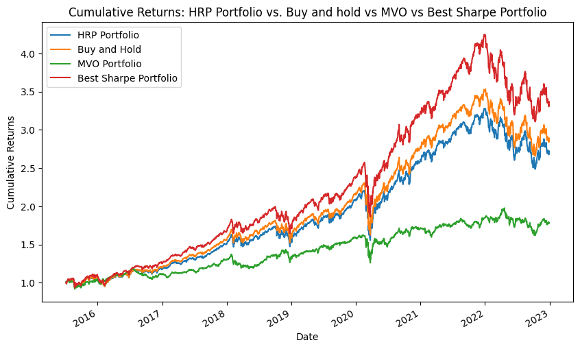HRP vs Buy and Hold vs MVO vs Best Sharpe Portfolio

The Best Sharpe Portfolio was created by creating an Efficient Frontier Report

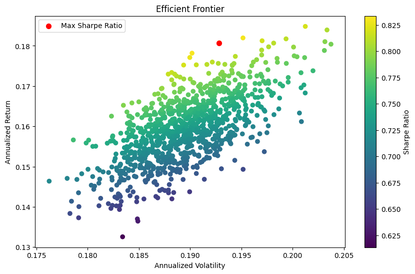Efficient Frontier Report

Evaluation of Results

Our analysis reveals some intriguing results. The Best Sharpe Portfolio, constructed based on the Efficient Frontier Report, leads the pack in terms of cumulative returns. The Buy and Hold strategy, which involves equal allocation to all selected stocks and holding them over the entire period, follows closely. Interestingly, the HRP strategy — known for its advanced approach to portfolio diversification — ranks third. Lastly, the MVO portfolio, based on the traditional mean-variance optimization, trails the group.

Delving into the Reasons

The superior performance of the Best Sharpe Portfolio can be attributed to its optimized asset allocation, which maximizes risk-adjusted returns. This strategy identifies the portfolio with the highest Sharpe Ratio on the Efficient Frontier, offering a favorable balance between expected return and risk.

The Buy and Hold strategy’s commendable performance is likely driven by the long-term bullish trend in the stock market over the observed period. By maintaining a steady position, investors would have reaped the benefits of the overall market rally.

The HRP portfolio, while delivering lower returns than the first two strategies, offers the advantage of enhanced risk management. HRP leverages hierarchical clustering to group assets based on their correlations, leading to more effective risk diversification. This strategy may prove valuable in turbulent market conditions.

MVO’s relatively lower performance may stem from several factors, including estimation errors in input parameters (mean returns and covariance matrix) and sensitivity to changing market conditions. MVO’s reliance on historical data for optimization could limit its adaptability to future market dynamics.

Conclusion

In this article, we embarked on a journey to compare two prominent investment strategies: Hierarchical Risk Parity (HRP) and Mean-Variance Optimization (MVO). Through our analysis, we observed that both strategies offer unique advantages and challenges in the pursuit of portfolio diversification and risk-adjusted returns.

Our results indicate that the HRP strategy, with its focus on hierarchical clustering and risk parity allocation, provides a more stable risk profile. By accounting for the hierarchical structure of asset correlations, HRP constructs a diversified portfolio that aims to equalize risk contributions, making it a valuable tool during market uncertainties.

On the other hand, the MVO strategy, underpinned by the principles of Modern Portfolio Theory, seeks to optimize asset allocation based on expected returns and risk. However, MVO’s performance is influenced by estimation errors in input parameters and sensitivity to changing market conditions. This sensitivity underscores the importance of regular rebalancing and careful estimation of input parameters.

Notably, the Best Sharpe Portfolio, derived from the Efficient Frontier, emerged as the top performer in our analysis. By optimizing the balance between risk and return, this portfolio achieved superior risk-adjusted performance, demonstrating the value of systematic optimization.

In conclusion, the choice between Hierarchical Risk Parity and Mean-Variance Optimization depends on investors’ objectives, risk tolerance, and market outlook. Both strategies have their place in the toolkit of a well-informed investor. As we assess their relative performance alongside the Best Sharpe Ratio, we are reminded that diversification — whether across assets or strategies — is a cornerstone of prudent investment practice.

Note: This article reflects a hypothetical analysis based on selected stocks from the S&P 500. Past performance is not indicative of future results. Investment decisions should be made based on careful research and consultation with financial advisors.

Colab Notebook Link

You can view and run all of the code used in this article here: Google Colaboratory Edit descriptioncolab.research.google.com

References

1. López de Prado, Marcos. “Chapter 16: Hierarchical Risk Parity.” In Advances in Financial Machine Learning, 261–283. Hoboken, NJ: John Wiley & Sons, 2018. https://www.wiley.com/en-us/Advances+in+Financial+Machine+Learning-p-9781119482086

2. Raffinot, Thomas. “Hierarchical Clustering Based Asset Allocation.” SSRN, 2017. https://papers.ssrn.com/sol3/papers.cfm?abstract_id=2840729

3. Snow, Derek, Machine Learning in Asset Management (July 16, 2019). JFDS: https://jfds.pm-research.com/content/2/1/10 , Available at SSRN: https://ssrn.com/abstract=3420952 or http://dx.doi.org/10.2139/ssrn.3420952

4. Chapter 16 Implementation by Aditya Vyas for FirmAI, https://colab.research.google.com/drive/1-Z3OjjnIR-41E2tycKFosvxEt-RrAgZB